|
TriTrack Air Drag Analysis
Investigation of the Flow About the TriTrack System
Amanda Kelly
Aaron Hamblin
Amanda Babcock
John Burroughs
Valori Booth
Fluids Lab ASE 120K
With Dr. David Goldstein
12/05/03
Department of Aerospace Engineering and Engineering Mechanics
University of Texas at Austin
W. R. Woolrich Laboratories
Austin, TX 78712
| |
Airflow over a 1/12 scaled model of the proposed TriTrack
system was investigated in the W.R. Woolrich laboratories
to determine the nature of the flow about the system and to
the drag coefficient of the vehicle. Jerry Roane, the inventor
of TriTrack, proposed the testing to support claims with empirical
data to Austin’s Board of Transportation. The complete
TriTrack system includes the vehicle body, two axles, two
wheels, and a triangular track. To determine the nature of
the flow about the vehicle, flow visualization was performed
with visible smoke released into the airstream and tufts placed
on the surface of the TriTrack system. At approximately 3.05
m/s, the smoke showed that the flow remained attached to the
body for almost its entire length. At about 18.29 m/s, the
tufts on the vehicle body depicted attached flow for the majority
of the vehicle by remaining streamlined. Drag coefficients
for the various system configurations were determined with
a force balance. The drag coefficient of the vehicle with
the entire system in place was calculated to be 0.15. The
wind tunnel tests revealed a drag coefficient of 0.07 for
the vehicle body alone, which was in agreement with Mr. Roane's
estimate of 0.09. By analyzing the drag coefficients for every
configuration, the axles and wheels were found to account
for approximately half of the drag of the system.
|
Table of Contents
- Abstract
- Nomenclature and Abbreviations
- Introduction
- Theory
- Methods
- Equations
- Apparatus and Test Procedure
- Flow Visualization
- Drag Coefficient
- Results
- Flow Visualization
- Smoke Wire
- Tufts
- Coefficient of Drag Determination
- Sphere
- Vehicle
- Conclusions
- References
- Figures
| |
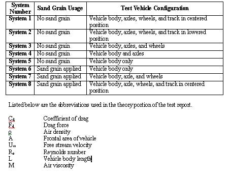
In Table 1 below a list is given of the nomenclature that
refers to each test vehicle configuration that was tested.
These system numbers will be used throughout the report.
Table 1 Description of System Configurations
| |
TriTrack is a monorail system proposed for the city of Austin
that has been in development since the 1973 Oil Embargo. A
local Austin inventor, Jerry Roane, has engineered the TriTrack
system to resolve several growing transportation concerns
for the general public. TriTrack is an electrically driven
vehicle that relieves the city of Austin of some of its dependence
on oil, an expensive natural resource that offers a limited
supply and produces dangerous byproducts to the environment.
The vehicle travels at about 37 mph on the residential streets
and about 180 mph on the monorail [1]. Collisions between
vehicles traveling above 37 mph have been shown to have a
high fatality rate, therefore, imposing this speed limit with
the TriTrack system will reduce road fatalities [1]. Clearance
between TriTrack vehicles on the monorail allows the vehicle
to safely accelerate to 180 mph. This system not only promotes
safety but it also provides the convenience of short travel
times.
The TriTrack vehicle body was selected carefully to be both
streamlined for efficiency and spacious for passengers. A
streamlined body, first designed in 1907, forces the air flow
to remain attached to the body, thereby eliminating the drag
associated with the air pressure that occurs in the wake behind
the separated flow [2]. The TriTrack vehicle is modeled after
the streamlined Class C Airship that has a body length to
diameter ratio of 4.62. Although ratios of 3.0 to 3.5 give
the smallest drag coefficients, a Class C Airship with the
ratio of 4.62 was proven by the Navy Aerodynamic Laboratory
in 1927 to have the lowest drag per unit volume [3], which
is essential for passengers.
Although the wind tunnel data taken in 1927
remains valid for the Class C Airship, slight differences
in the body design for the TriTrack vehicle warrant updated
wind tunnel tests. Jerry Roane fabricated a smoothed model
with high-end CAD equipment and machined it to within +/-
.05 mm of the data provided in the Navy’s report, making
a better model than the airship tested years ago. The TriTrack
vehicle also includes two axles and two wheels and excludes
a triangular section of the body where the railing will be
fitted. Another distinction between the two vehicles is that
the Navy's wind tunnel testing only went up to only
60 mph while the TriTrack vehicle is intended to travel at
180 mph.
Due to the deviation of the TriTrack model from
the Class C Airship, preliminary wind tunnel testing in the
W.R Woolrich Laboratories was necessary to get a better estimate
of the drag coefficient and flow behavior about the TriTrack
model. Because wind tunnel speeds are limited to 24.38 m/s
at the W.R Woolrich Laboratories, further testing will be
conducted at a later time at Pickle Laboratory to complement
the preliminary results.
| |
Flow visualization can be accomplished by the use of smoke
wire and tufts. The smoke wire is a visualization technique
that creates a sheet of smoke that passes over a test section.
The separation point of the flow is indicated by the point
where the smoke ceases to follow the contours of the body.
This wire is only effective for low speeds of 3.05 m/s or
less. Another technique of flow visualization is tufts, which
are short sections of twine attached to the body. The tufts
lay flat and smooth along the test article when subject to
laminar flow and are greatly disturbed in the presence of
turbulent flow. The point at which the tufts transition from
stable to disturbed is the separation point.
A force balance is a component used to measures
normal and tangential forces exerted on a body by aerodynamic
resistance. The forces can then be used to calculate lift
and drag coefficients. Sand grain can be applied to a vehicle
to force super-critical flow. Super-critical flow has turbulent
boundary layer that re-energizes the flow and causes the separation
point to move farther back on the body. The region of separated
flow has less contact with the body in super-critical flow,
which subsequently lowers the drag coefficient.
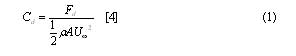
The Coefficient of Drag (Cd) is a dimensionless ratio of drag
force to dynamic force. It can be attained using the momentum
equation applied to the control volume of the wind tunnel
test section and assuming steady, incompressible flow. After
the drag force is found, the drag coefficient can be calculated
through the following equation:
The Reynolds Number (Re) for the vehicle can also be critical
to the results. It is a relation of the laminar to turbulent
transition point to the boundary layer thickness and skin
friction of the test article [2]. Re is dependent on the free
stream velocity. To better ensure the Reynolds Number obtained
is accurate sand grain is added to the nose of the vehicle.
When sand grain is applied to the nose, a Reynolds Number
is obtained that simulates a faster free stream. The vehicle
is designed to be traveling at speeds of up to 80.47 m/s but
the testing of the vehicle is done at a maximum free stream
velocity of 24.38 m/s. Reynolds Number equals:
| |
Flow visualization and data acquisition were performed in
the subsonic, open-test section wind tunnel at the University
of Texas at Austin. Several different configurations of the
experimental TriTrack vehicle and track were tested to determine
the nature of the flow around the system and the drag coefficient
of each configuration. The vehicle, provided by Jerry Roane
of Roane Inventions, was modeled after a Class C airship which
is the basic shape of a blimp. The body was machined from
billet aluminum measuring 0.44 m long with a maximum diameter
of 0.10 m located 0.16 m from the nose. Each of the two spun
aluminum wheels had an area of 4.23 x 10⁻⁴ m2 and each of
the two aluminum axles had an area of 3.58 x 10⁻⁴ m2. In order
to accommodate the triangular track, a 1.89 x 10⁻⁴ m2 triangular
sector was removed from the bottom of the vehicle.
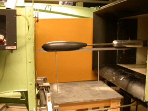
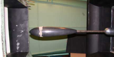
The vehicle was mounted in the wind tunnel on a rear-mounted
sting. The track, supported by a platform, was positioned
under the vehicle as shown in Figure 1. Flow visualization
was first performed with a smoke wire at low flow speeds of
about 3.05 m/s. The flow was examined over the vehicle and
the wheels in system 1 to determine the exact separation point.
Smoke visualization was repeated for system 5 in order to
analyze the flow over only the vehicle body. The approximate
separation point of the flow around the vehicle in system
1 at higher flow speed was determined by observing tufts attached
to the vehicle, wheels and track. The behavior of the flow
near the track and vehicle junction was also examined with
the tufts. Tuft visualization was then repeated for system
5. Digital pictures were taken with a camera provided by the
Aerospace Engineering Learning Resource Center for both visualization
techniques.
The drag coefficients for several different configurations
were then calculated using the tangential force measurements
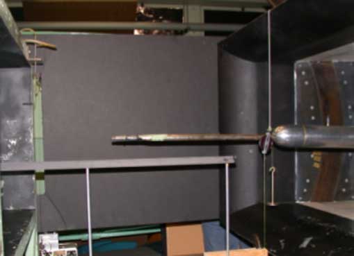
obtained from a force balance. In order to calibrate the force
balance, known tangential forces were applied to the sting
with a string and pulley assembly, as shown in Figure 2.
The axial force measured by the force balance was sent to a computer
with a data acquisition system. After calibrating the force
balance, a metal sphere with a diameter of 0.10 m was mounted
on the force balance and drag force measurements were taken
at various flow speeds. A drag coefficient for the sphere
was calculated from the drag force data and compared to known
values of drag coefficient to ensure the accuracy of the force
balance. The vehicle was then mounted on the force balance
and the track was placed directly beneath, but not contacting,
the vehicle. The track did not contact the vehicle so that
no loads were transmitted to the force balance by the track.
Twenty drag force measurements were taken at zero free stream
velocity to establish a zero force value. Twenty measurements
were then taken for increasing flow speeds between 3.05 m/s
and 24.38 m/s at 1.52 m/s intervals. For each flow speed,
the drag coefficient was calculated by dividing the average
of the drag force measurements at that flow speed by the frontal
area of the configuration. A plot of drag coefficient versus
free stream velocity was created to determine the drag coefficient
for that configuration. The same procedure was repeated for
systems 2 through 5 after removing the track, again after
removing the wheels, and for a fourth time after removing
the axles. Sand grain roughness was then applied to the maximum
diameter of the vehicle and the procedure was performed for
systems 6 through 8 to determine if forcing the flow over
the vehicle to become super critical would lower the drag
coefficient.
| |
Testing of the TriTrack was partitioned into two sections:
flow visualization and coefficient of drag determination.
Two techniques were used to visualize the flow about the TriTrack
test vehicle. A smoke wire created a vertical profile of the
flow about the test subject.
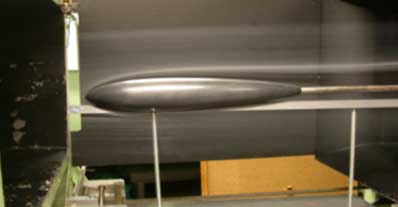
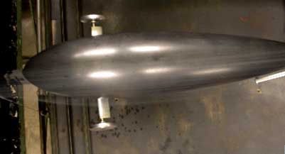
Flow was first tested over the TriTrack body placed atop the
triangular track. The smoke showed a very laminar flow over
the entire vehicle with minimal disturbances from the track.
The flow remained attached to the vehicle for almost the entire
length of the body. The attached flow as well as a clearly
defined stagnation point can be seen in Figure 3.
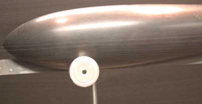
In order to visualize the flow about the TriTrack
wheels, the model was assembled into the system 1 configuration
shown in Figure 4 and the smoke wire was positioned
directly in front of the wheel position. Figure 4 shows
the flow about a wheel. The wake created behind the circular surface was
very minimal and could only be observed on the lower portion
of the wheel. A top view of the flow about a wheel is shown
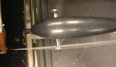
in Figure 5. The symmetric airfoil shaped axles of
TriTrack proved to be a very aerodynamically smooth shape as presented
in Figure 6. The flow remained attached to the axle and
extremely little disturbance was seen at the trailing edge. Smoke
visualization from the top view for the system1 configuration, can be seen
in Figure 7. Flow was closely attached to the body and
any disturbed wake by the axles was not observable from this view.
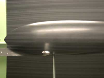
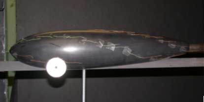
Tufts placed in a spiral pattern on the TriTrack body were
used for flow visualization at a free stream velocity of 18.29
m/s. The tufts in Figure 8 are straight and pointed
directly downstream. Static tufts are visual indicator of laminar flow
which agrees with the smoke visualization technique. Even
tufts placed on the top surface of the airfoil axle were stable.
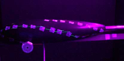
Very slight disturbance was observed from the tuft placed
on the top of the wheel. The disturbance can best be seen
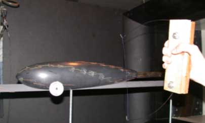
in the black lit image in Figure 9. A tuft wand was
used to try to determine a flow separation point but no disturbance
of tufts were observed over the entire structure. A view of
the tuft wand testing can be seen in Figure 10.
Utilizing the force balance, both the sphere and the vehicle
were tested for their average drag coefficients at varying
free stream velocities. For the vehicle, eight systems were
tested. The system configurations are described in Table 1.
Figure 11 is a plot of the coefficient of drag
versus free stream velocity for the sphere. The trend line represents
an estimated average of the data. To obtain a better fitting
curve, the experimental high and low anomalies were discarded
in the calculation of the trend line. The average value from
this trend line is 0.57. White states that the accepted average
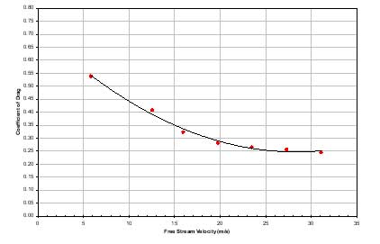
coefficient of drag for a sphere is 0.47 [4]. A plot of the
drag coefficient for the sphere with the addition of sand
grain is shown in Figure 12. The trend line from this
data set yields a rough average of 0.35. The addition of sand grain
lowered the average drag coefficient, confirming turbulent
flow transition. The accepted value of drag coefficient for
turbulent flow about a sphere is 0.20 [4]. The differences
between the calculated drag coefficients and the universally
accepted values confirmed the presence of sting drag.
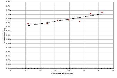
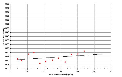
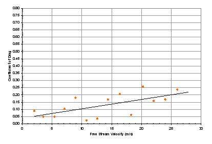
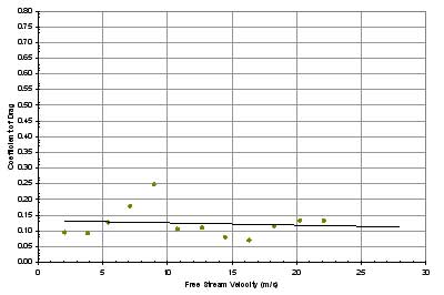
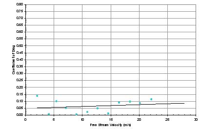
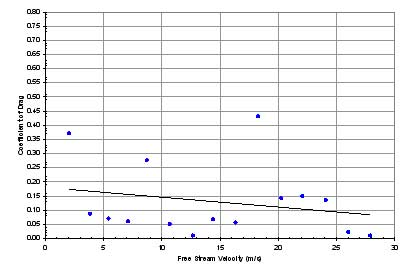
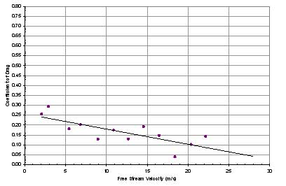
Figure 13 through Figure 20
are plots of drag coefficient versus free stream velocity for the data in
their respective experiments. Average values, taken from the trend lines for
each set of data, are shown for each system in the following
table.
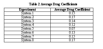
In systems 1 through 5, two trends became apparent.
First, the drag coefficients were very low, nearing 0.10 on
average. Second, removing the wheels and axles significantly
lowered the average drag coefficient. With the loss of the
wheels in system 4 and the axles in system 5, the drag coefficient
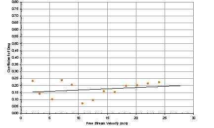
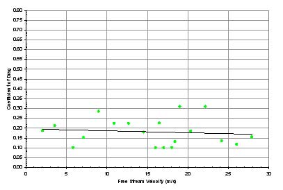
dropped by half. With the addition of sand grain in systems
6 through 8, as shown in Figure 21, a turbulent
boundary layer was induced in an attempt to lower the vehicle's drag
coefficient. However, the sand grain seemed to raise the drag
coefficient on average. Parallel experiments of systems 5
and 6 saw an average drag coefficient increase of 0.05. Systems
3 and 7 showed an increase of 0.01, and systems 1 and 8 showed
a 0.02 increase. Another point of interest was the removal
of the track. Findings from track removal showed a uniform
decrease in the average estimated drag coefficient. The decreases
in the system changes from 8 to 7 and 1 to 3 were 0.01 and
0.03, respectively.
Finally, as observed in the sphere experiment,
there was sting drag present. Each drag coefficient in Table
2 would be higher than the measured value due to added drag
caused by the sting. Also, the wire used to support the weight
of the vehicle created a small amount of drag. Large variations
in the measurements taken due to force balance oscillation
observed at high free stream velocities render the drag of
the wire too small to affect our calculations.
| |
The results of the flow visualization showed laminar flow
across almost the entire vehicle, as expected from the research
conducted on the Class C airship. The triangular sector removed
from the vehicle for the track did not cause significant changes
in the flow, as expected. During calibration, the calculated
average coefficient of drag for the sphere was higher than
the nominal value due to drag force on the sting and calibration
errors. However, the values were similar enough to ensure
that the force balance was providing accurate data. The expected
drag coefficient for system 5 was 0.09 due to small differences
between the TriTrack vehicle and the Class C airship. The
measured drag coefficient for system 5 was 0.07, which was
close to the expected value. Some random errors may have resulted
from oscillation of the vehicle, which originated from motor-induced
tunnel vibration. Because flow about the vehicle without sand
grains stayed attached for almost the entire length of the
vehicle, forcing supercritical flow with sand grains did not
change the separation point enough to reduce an already negligible
pressure drag. In fact, when sand grains were applied to the
vehicle in systems 6 through 8, the coefficient of drag increased
because of the added friction drag from the sand. For system
3, the drag coefficient was found to be almost twice as large
as the drag coefficient for system 5, meaning that the wheels
and axles account for half of the drag of the vehicle. As
suggested by Mr. Roane, the performance of the TriTrack system
could be greatly improved if the wheels were retractable.
|
- Roane, Jerry, “TriTrack,” http://www.tritrack.net,
23 November 2003.
- Von Mises, R., Theory of Flight, Dover Publications, New
York, 1959, pp. 102.
- NACA, “Drag of C-class airship hulls of various fineness ratios,” http://naca.larc.nasa.gov/reports/1929/naca-report-291/naca-report-291.pdf, 26 November 2003.
- White, F., Fluid Mechanics, 5th ed., Avenues of Americas, New York, 2003, pp. 25, 314, 48
|
|
|